")
Contemplate a worksheet that has tens of hundreds of rows of knowledge. Just by wanting on the uncooked knowledge – patterns and developments can be very troublesome to identify. Conditional formatting provides an additional technique of visualizing knowledge and enhancing worksheet comprehension, very like charts.
What’s Conditional Formatting in Excel?
Conditional Formatting is a function in an Excel spreadsheet. It’s used to simply preserve the standing of the consequence. It’s most frequently used as color-based formatting to spotlight, emphasize, or differentiate amongst knowledge and data saved in an Excel spreadsheet.
In relation to making use of different types to knowledge that matches explicit standards, Excel conditional formatting is a extremely helpful function. It may well make it simpler so that you can draw consideration to the important thing particulars in your spreadsheets and shortly establish variations in cell values.
Varieties/Conditional Formatting Presets
You should utilize preset guidelines, together with Shade scales, Information Bars, Icon Units, Kind filter, and many others. to conditionally format your knowledge, or you possibly can assemble your personal guidelines that specify when and the way the chosen cells ought to be highlighted.
- Information Bars, Much like a bar graph, knowledge bars are horizontal bars which might be added to every cell
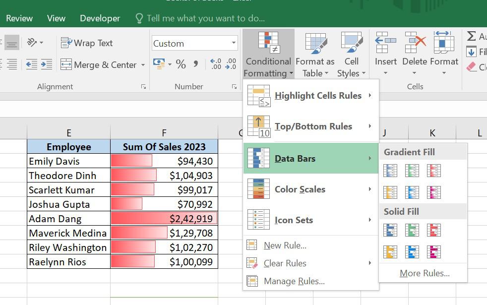
Information Bars
- Shade scales alter every cell’s shade relying on its worth. A two- or three-color gradient is used for every shade scale
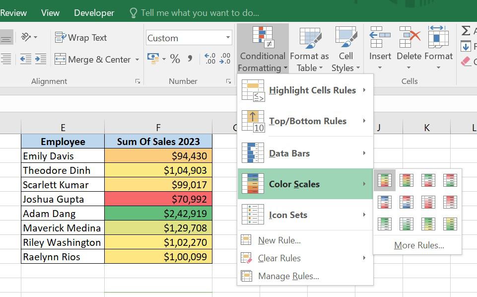
Shade scales
- Icon Units, primarily based on the worth of every cell, icon units assign a definite icon to every cell.
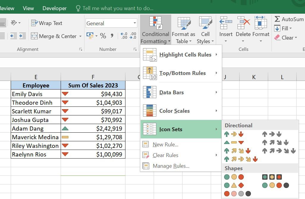
Icon Units
The place To Discover Conditional Formatting in Excel
Conditional formatting is obtainable from Excel 2010 via Excel 365 in the identical location.
House tab > Types group > Conditional formatting.
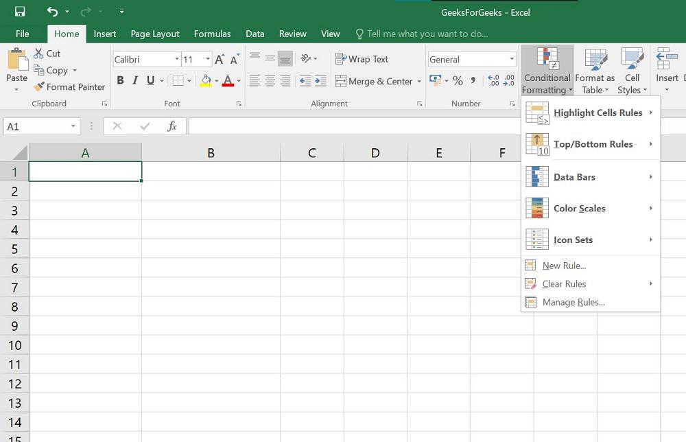
Conditional Formatting in Excel
How you can Use Conditional Formatting in Excel
Steps to make the most of Excel conditional formatting are as follows:
Step 1. Choose the Cells
Choose the cells you need to format within the Spreadsheet
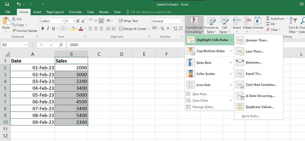
Step 2. Click on on Conditional Formatting
Click on Conditional Formatting, On the House tab, within the Types group
Step 3. From a Set of Preset Guidelines, Choose the Required One
From a set of preset guidelines, choose the one which finest serves your wants
Utilizing Conditional Formatting In Excel
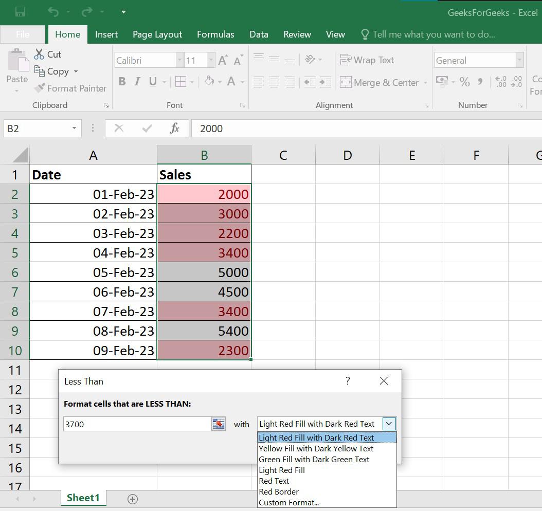
Step 4. Enter the Worth and Choose the Chosen Format from the Drop-Down Record
Enter the worth within the field on the left of the dialogue field and choose the chosen format from the drop-down record on the fitting (with Default Mild Purple Fill with Darkish Purple Textual content)
Utilizing Conditional Formatting In Excel
Different rule sorts that may be applicable to your knowledge, comparable to:
- Better than or equal to
- Between two values
- Textual content that accommodates particular phrases or characters
- Date occurring in a sure vary
- Duplicate values
How you can Use a Preset Rule with Customized Formatting
You may choose every other shade for the background, textual content, or borders of the cells if none of the usual layouts appeals to you. That is how:
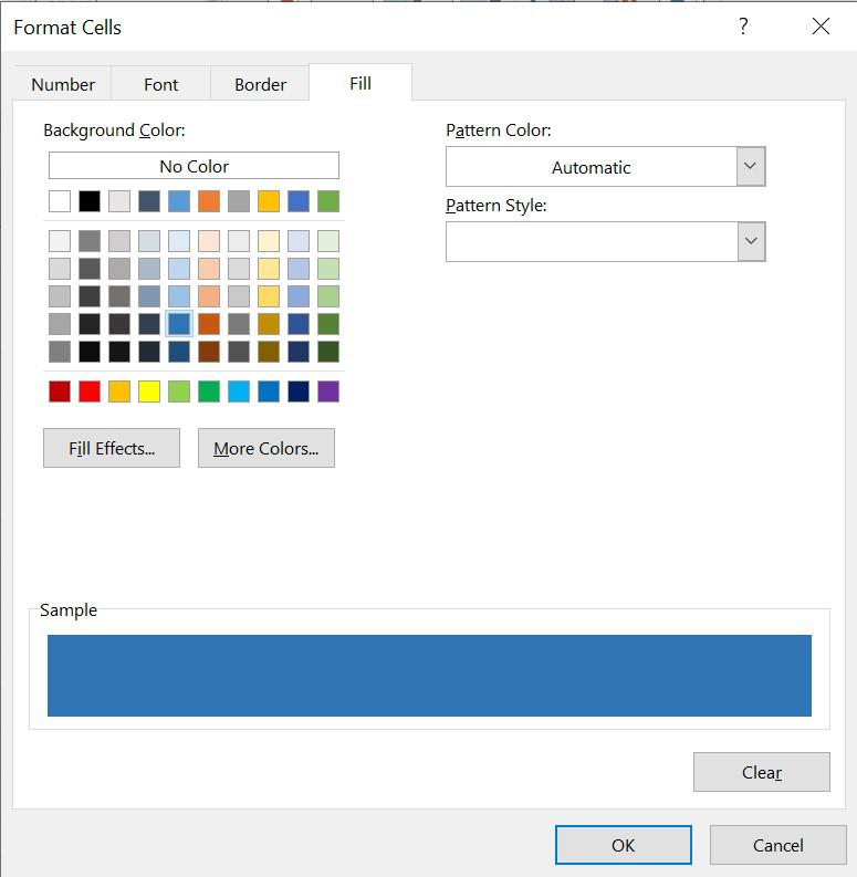
Step 1. Choose Customized Format, Within the preset rule dialogue field, from the drop-down record on the fitting
Step 2. Change between the Font, Border, and Fill tabs within the Format Cells dialogue window to pick the popular font model, border model, and background shade, respectively, click on OK
Customized formatting
Step 3. Click on OK to use the customized formatting of your selection
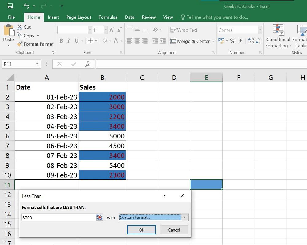
Customized formatting
How you can Create a New Conditional Formatting Rule in Excel
You may create a brand new Conditional Formatting Rule in Excel from scratch. To take action, comply with these steps:
Step 1. Choose the cells to be formatted and click on Conditional Formatting > New Rule.
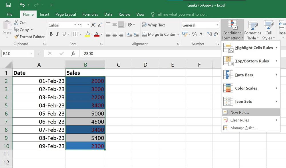
New Conditional Formatting Rule in Excel
Step 2. Choose the rule sort, within the New Formatting Rule dialog field
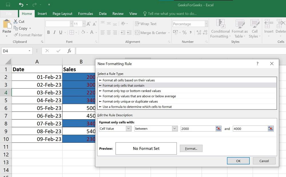
New Conditional Formatting Rule in Excel
Step 3. Click on the Format button, and select the colour you need to fill.
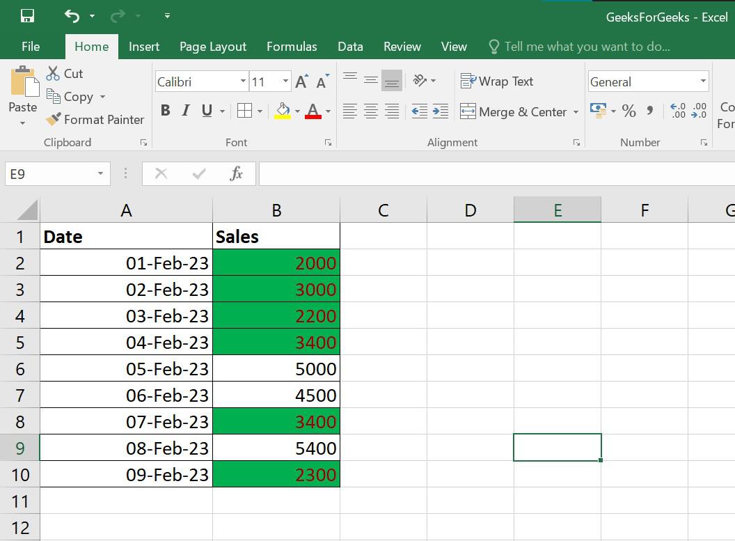
New Conditional Formatting Rule in Excel
Step 4. Click on OK and your New conditional formatting is finished!
How you can Edit Conditional Formatting Guidelines in Excel
To make any modifications in an already current Formatting Rule in Excel, comply with these steps:
Step 1. Choose any cell to which a rule already applies, Click on on Handle Guidelines beneath Conditional Formatting
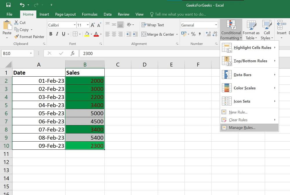
Enhancing Conditional Formatting Guidelines in Excel
Step 2. This can open the Guidelines Supervisor dialog field, choose the rule you need to modify, then Click on on Edit Rule.
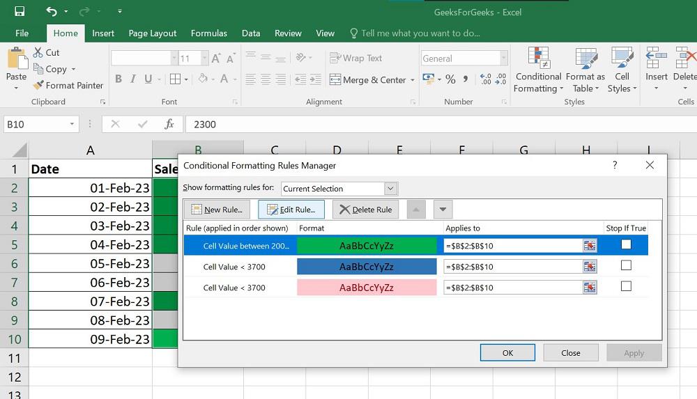
Enhancing Conditional Formatting Guidelines in Excel
Step 3. Make the required modifications within the Edit Formatting Rule dialogue window, Click on on Okay
Excel Conditional Formatting Examples:
Some State of affairs-Based mostly Examples of Conditional Formatting in Excel:
State of affairs 1. Figuring out Duplicates
Steps to figuring out duplicate values:
Step 1: Choose the cells the place you need to establish duplicate values. For instance: choose the column TOT as proven within the determine.

Step 2: Click on on the Conditional Formatting and click on on new guidelines. Now a window seems, choose ‘format solely distinctive and duplicate values’ and click on on the format.

Step 3: Choose the Fill choice within the tab and select the background shade and click on okay.

Step 4: Now the duplicate values as proven within the determine.

State of affairs 2. Cell Highlighting with Worth Better or Lower than a Quantity
Observe the beneath steps for highlighting cells with a worth better or lower than a given quantity:
Step 1: Choose the cells that you just need to spotlight with Better or lower than a quantity.

Step 2: Click on on the conditional formatting and click on on new guidelines. Now choose “Format all cells primarily based on their values“. Within the ‘Minimal’ and select the worth you need to establish the lesser values and select the colour. Equally, Within the Most and select the worth you need to establish the lesser values and select the colour. And click on okay.

Step 3: Within the beneath determine, the values with inexperienced shade point out better values and the values with pink shade point out fewer values.

State of affairs 3. Highlighting High or Backside N Objects
To spotlight the highest and/or the underside N gadgets choose the cells the place you need to spotlight high and backside N gadgets and click on on the conditional formatting->High/backside cells->High 10 Objects. Select a worth in format cells that rank on the high and select the format and click on okay.
Within the beneath determine, the pink shade signifies the highest 5 values in rank.

How you can Copy Excel Conditional Formatting
You gained’t want to begin over when making use of a conditional format you’ve already established to totally different knowledge. To switch the present conditional formatting rule(s) to a different knowledge assortment, simply make the most of Format Painter.
Step 1. Select the cell whose conditional formatting you need to duplicate
Step 2. Click on on Format Painter beneath House
Step 3. Click on on the primary cell within the vary you need to format, then drag the paintbrush all the way down to the final cell to stick the copied formatting
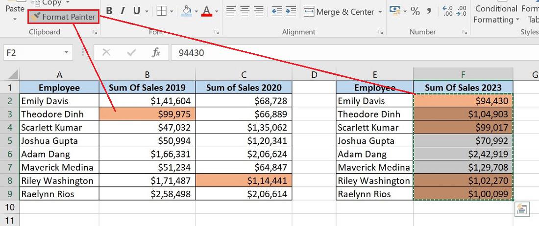
Copy Excel Conditional Formatting
Step 4. To cease utilizing the paintbrush, press Esc.
How you can Delete Conditional Formatting Guidelines
There are two simple methods to delete conditional formatting guidelines
1. Select your best option after deciding on the specified cell vary and clicking Conditional Formatting > Clear Guidelines
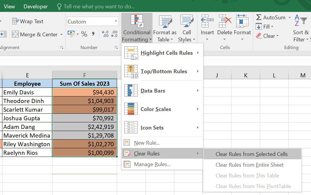
Deleting conditional formatting guidelines
2. Choose the rule and click on the Delete Rule button, Underneath the Conditional Formatting Guidelines Supervisor
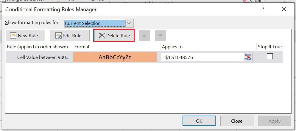
Deleting conditional formatting guidelines
FAQs on Excel Conditional Formatting
Listed below are among the most ceaselessly requested questions on Excel Conditional Formatting
1. What are the three conditional formatting choices?
Three classes have been established for Conditional Formatting in Excel.
- Much like a bar graph, Information bars are horizontal bars which might be added to every cell
- Shade scales alter every cell’s shade relying on its worth. A two- or three-color gradient is used for every shade scale
- Icon Units, primarily based on the worth of every cell, icon units assign a definite icon to every cell
2. Can I copy Conditional Formatting to different cells in Excel?
Sure, we are able to copy Conditional Formatting to different cells in Excel. There are a number of methods to repeat the conditional formatting to different cells, comparable to –
- Easy copy-paste
- Copy and paste conditional formatting solely
- Utilizing the format painter
3. How do I take away Conditional Formatting from cells in Excel?
To take away the chosen vary conditional formatting, please comply with the below-mentioned steps:
- Choose the vary that you just need to take away the conditional formatting from
- Click on House > Conditional Formatting > Clear Guidelines > Clear Guidelines from Chosen Cells
4. Can I exploit icons or knowledge bars in Conditional Formatting?
Sure, you should utilize Icons or Information bars in Conditional Formatting in Excel. To make use of both of those, comply with the beneath steps:
- Choose the vary that you just need to apply the conditional formatting to
- Click on on Conditional Formatting on the House Tab
- Level to Information Bars, and select from gradient fill or stable fill or Level to Icon units and select your required icons
5. Can I apply Conditional Formatting primarily based on one other cell’s worth in Excel?
You need to use system in the event you want to format a complete row relying on the worth of a single cell or apply conditional formatting primarily based on one other cell.
