Close to-real-time fraud detection utilizing Amazon Redshift Streaming Ingestion with Amazon Kinesis Knowledge Streams and Amazon Redshift ML

The significance of information warehouses and analytics carried out on information warehouse platforms has been growing steadily through the years, with many companies coming to depend on these programs as mission-critical for each short-term operational decision-making and long-term strategic planning. Historically, information warehouses are refreshed in batch cycles, for instance, month-to-month, weekly, or day by day, so that companies can derive numerous insights from them.

Many organizations are realizing that near-real-time information ingestion together with superior analytics opens up new alternatives. For instance, a monetary institute can predict if a bank card transaction is fraudulent by operating an anomaly detection program in near-real-time mode somewhat than in batch mode.

On this submit, we present how Amazon Redshift can ship streaming ingestion and machine studying (ML) predictions multi functional platform.

Amazon Redshift is a quick, scalable, safe, and totally managed cloud information warehouse that makes it easy and cost-effective to investigate all of your information utilizing customary SQL.

Amazon Redshift ML makes it simple for information analysts and database builders to create, practice, and apply ML fashions utilizing acquainted SQL instructions in Amazon Redshift information warehouses.

We’re excited to launch Amazon Redshift Streaming Ingestion for Amazon Kinesis Knowledge Streams and Amazon Managed Streaming for Apache Kafka (Amazon MSK), which lets you ingest information straight from a Kinesis information stream or Kafka subject with out having to stage the information in Amazon Easy Storage Service (Amazon S3). Amazon Redshift streaming ingestion means that you can obtain low latency within the order of seconds whereas ingesting lots of of megabytes of information into your information warehouse.

This submit demonstrates how Amazon Redshift, the cloud information warehouse means that you can construct near-real-time ML predictions through the use of Amazon Redshift streaming ingestion and Redshift ML options with acquainted SQL language.

Answer overview

By following the steps outlined on this submit, you’ll have the ability to arrange a producer streamer utility on an Amazon Elastic Compute Cloud (Amazon EC2) occasion that simulates bank card transactions and pushes information to Kinesis Knowledge Streams in actual time. You arrange an Amazon Redshift Streaming Ingestion materialized view on Amazon Redshift, the place streaming information is acquired. You practice and construct a Redshift ML mannequin to generate real-time inferences towards the streaming information.

The next diagram illustrates the structure and course of circulate.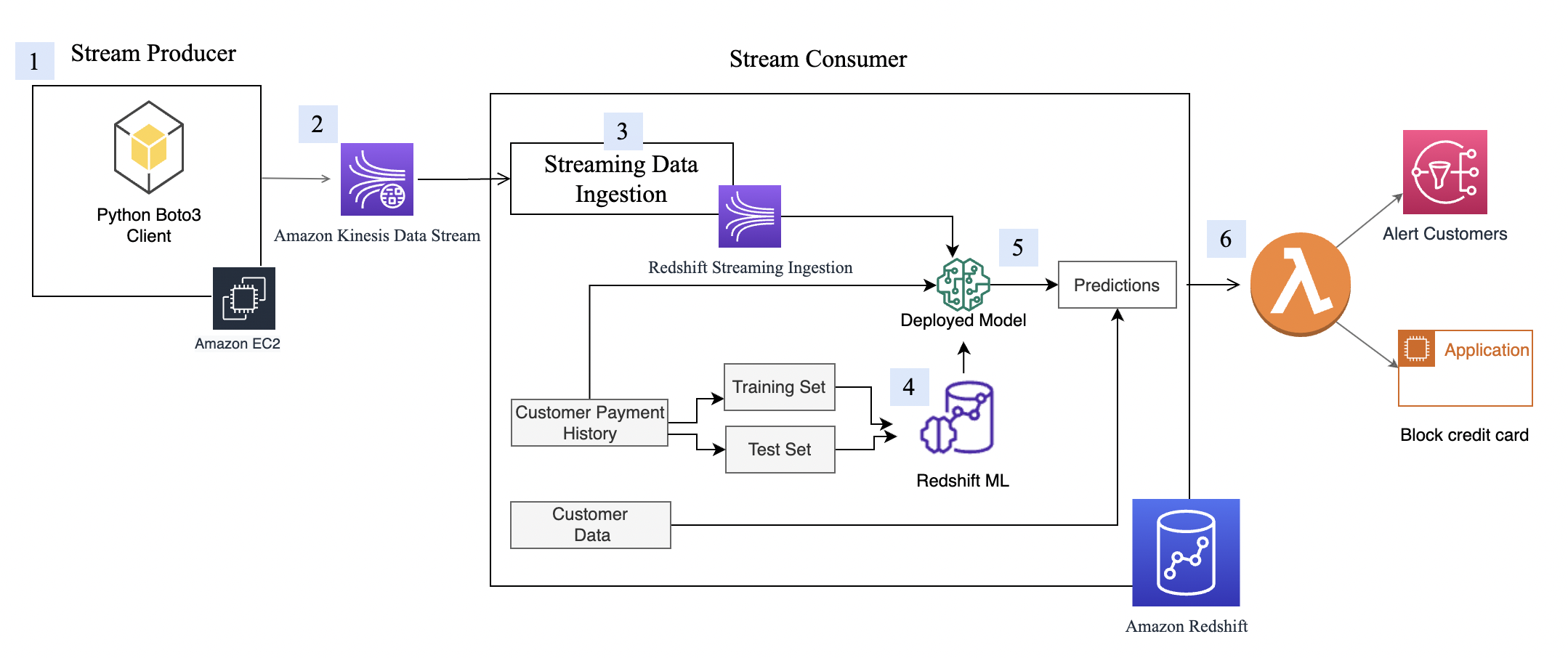

The step-by-step course of is as follows:

1. The EC2 occasion simulates a bank card transaction utility, which inserts bank card transactions into the Kinesis information stream.
2. The info stream shops the incoming bank card transaction information.
3. An Amazon Redshift Streaming Ingestion materialized view is created on prime of the information stream, which routinely ingests streaming information into Amazon Redshift.
4. You construct, practice, and deploy an ML mannequin utilizing Redshift ML. The Redshift ML mannequin is skilled utilizing historic transactional information.
5. You rework the streaming information and generate ML predictions.
6. You may alert prospects or replace the appliance to mitigate danger.

This walkthrough makes use of bank card transaction streaming information. The bank card transaction information is fictitious and relies on a simulator. The shopper dataset can also be fictitious and is generated with some random information capabilities.

Conditions

1. Create an Amazon Redshift cluster.
2. Configure the cluster to make use of Redshift ML.
3. Create an AWS Identification and Entry Administration (IAM) person.
4. Replace the IAM function hooked up to the Redshift cluster to incorporate permissions to entry the Kinesis information stream. For extra details about the required coverage, confer with Getting began with streaming ingestion.
5. Create an m5.4xlarge EC2 occasion. We examined Producer utility with m5.4xlarge occasion however you’re free to make use of different occasion kind. When creating the occasion, use the amzn2-ami-kernel-5.10-hvm-2.0.20220426.0-x86_64-gp2 AMI.
6. To ensure that Python3 is put in within the EC2 occasion, run the next command to verity your Python model (be aware that the information extraction script solely works on Python 3):

7. Set up the next dependent packages to run the simulator program:

sudo yum set up python3-pip
pip3 set up numpy
pip3 set up pandas
pip3 set up matplotlib
pip3 set up seaborn
pip3 set up boto3

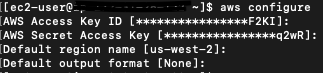
8. Configure Amazon EC2 utilizing the variables like AWS credentials generated for IAM person created in step 3 above. The next screenshot exhibits an instance utilizing aws configure.

Arrange Kinesis Knowledge Streams

Amazon Kinesis Knowledge Streams is a massively scalable and sturdy real-time information streaming service. It will possibly constantly seize gigabytes of information per second from lots of of 1000’s of sources, equivalent to web site clickstreams, database occasion streams, monetary transactions, social media feeds, IT logs, and location-tracking occasions. The info collected is offered in milliseconds to allow real-time analytics use instances equivalent to real-time dashboards, real-time anomaly detection, dynamic pricing, and extra. We use Kinesis Knowledge Streams as a result of it’s a serverless answer that may scale based mostly on utilization.

Create a Kinesis information stream

First, it’s worthwhile to create a Kinesis information stream to obtain the streaming information:

1. On the Amazon Kinesis console, select Knowledge streams within the navigation pane.
2. Select Create information stream.
3. For Knowledge stream identify, enter cust-payment-txn-stream.
4. For Capability mode, choose On-demand.
5. For the remainder of the choices, select the default choices and comply with via the prompts to finish the setup.
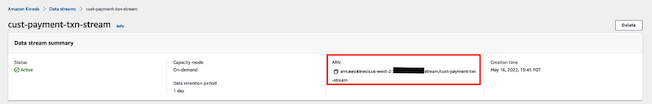
6. Seize the ARN for the created information stream to make use of within the subsequent part when defining your IAM coverage.

Arrange permissions

For a streaming utility to write down to Kinesis Knowledge Streams, the appliance must have entry to Kinesis. You need to use the next coverage assertion to grant the simulator course of that you just arrange in subsequent part entry to the information stream. Use the ARN of the information stream that you just saved within the earlier step.

{
"Model": "2012-10-17",
"Assertion": [
{
"Sid": "Stmt123",
"Effect": "Allow",
"Action": [
"kinesis:DescribeStream",
"kinesis:PutRecord",
"kinesis:PutRecords",
"kinesis:GetShardIterator",
"kinesis:GetRecords",
"kinesis:ListShards",
"kinesis:DescribeStreamSummary"
],
"Useful resource": [
"arn:aws:kinesis:us-west-2:xxxxxxxxxxxx:stream/cust-payment-txn-stream"
]
}
]
}

Configure the stream producer

Earlier than we are able to eat streaming information in Amazon Redshift, we want a streaming information supply that writes information to the Kinesis information stream. This submit makes use of a custom-built information generator and the AWS SDK for Python (Boto3) to publish the information to the information stream. For setup directions, confer with Producer Simulator. This simulator course of publishes streaming information to the information stream created within the earlier step (cust-payment-txn-stream).

Configure the stream client

This part talks about configuring the stream client (the Amazon Redshift streaming ingestion view).

Amazon Redshift Streaming Ingestion gives low-latency, high-speed ingestion of streaming information from Kinesis Knowledge Streams into an Amazon Redshift materialized view. You may configure your Amazon Redshift cluster to allow streaming ingestion and create a materialized view with auto refresh, utilizing SQL statements, as described in Creating materialized views in Amazon Redshift. The automated materialized view refresh course of will ingest streaming information at lots of of megabytes of information per second from Kinesis Knowledge Streams into Amazon Redshift. This ends in quick entry to exterior information that’s shortly refreshed.

After creating the materialized view, you’ll be able to entry your information from the information stream utilizing SQL and simplify your information pipelines by creating materialized views straight on prime of the stream.

Full the next steps to configure an Amazon Redshift streaming materialized view:

1. On the IAM console, select insurance policies within the navigation pane.
2. Select Create coverage.
3. Create a brand new IAM coverage known as KinesisStreamPolicy.  For the streaming coverage definition, see Getting began with streaming ingestion.
4. Within the navigation pane, select Roles.
5. Select Create function.
6. Choose AWS service and select Redshift and Redshift customizable.
7. Create a brand new function known as redshift-streaming-role and fasten the coverage KinesisStreamPolicy.
8. Create an exterior schema to map to Kinesis Knowledge Streams :

CREATE EXTERNAL SCHEMA custpaytxn
FROM KINESIS IAM_ROLE 'arn:aws:iam::386xxxxxxxxx:function/redshift-streaming-role';

Now you’ll be able to create a materialized view to eat the stream information. You need to use the SUPER information kind to retailer the payload as is, in JSON format, or use Amazon Redshift JSON capabilities to parse the JSON information into particular person columns. For this submit, we use the second technique as a result of the schema is effectively outlined.

9. Create the streaming ingestion materialized view cust_payment_tx_stream. By specifying AUTO REFRESH YES within the following code, you’ll be able to allow automated refresh of the streaming ingestion view, which saves time by avoiding constructing information pipelines:

CREATE MATERIALIZED VIEW cust_payment_tx_stream
AUTO REFRESH YES
AS
SELECT approximate_arrival_timestamp ,
partition_key,
shard_id,
sequence_number,
json_extract_path_text(from_varbyte(kinesis_data, 'utf-8'),'TRANSACTION_ID')::bigint as TRANSACTION_ID,
json_extract_path_text(from_varbyte(kinesis_data, 'utf-8'),'TX_DATETIME')::character(50) as TX_DATETIME,
json_extract_path_text(from_varbyte(kinesis_data, 'utf-8'),'CUSTOMER_ID')::int as CUSTOMER_ID,
json_extract_path_text(from_varbyte(kinesis_data, 'utf-8'),'TERMINAL_ID')::int as TERMINAL_ID,
json_extract_path_text(from_varbyte(kinesis_data, 'utf-8'),'TX_AMOUNT')::decimal(18,2) as TX_AMOUNT,
json_extract_path_text(from_varbyte(kinesis_data, 'utf-8'),'TX_TIME_SECONDS')::int as TX_TIME_SECONDS,
json_extract_path_text(from_varbyte(kinesis_data, 'utf-8'),'TX_TIME_DAYS')::int as TX_TIME_DAYS
FROM custpaytxn."cust-payment-txn-stream"
The place is_utf8(kinesis_data) AND can_json_parse(kinesis_data);

Observe that json_extract_path_text has a size limitation of 64 KB. Additionally from_varbye filters information bigger than 65KB.

10. Refresh the information.

The Amazon Redshift streaming materialized view is auto refreshed by Amazon Redshift for you. This manner, you don’t want fear about information staleness. With materialized view auto refresh, information is routinely loaded into Amazon Redshift because it turns into accessible within the stream. When you select to manually carry out this operation, use the next command:

REFRESH MATERIALIZED VIEW cust_payment_tx_stream ;

11. Now let’s question the streaming materialized view to see pattern information:

Choose * from cust_payment_tx_stream restrict 10;

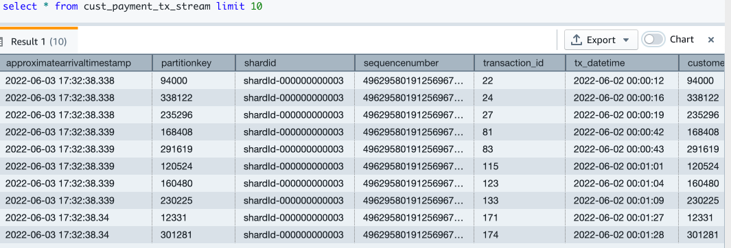
12. Let’s test what number of information are within the streaming view now:

Choose rely(*) as stream_rec_count from cust_payment_tx_stream;

Now you might have completed organising the Amazon Redshift streaming ingestion view, which is constantly up to date with incoming bank card transaction information. In my setup, I see that round 67,000 information have been pulled into the streaming view on the time once I ran my choose rely question. This quantity might be completely different for you.

Redshift ML

With Redshift ML, you’ll be able to convey a pre-trained ML mannequin or construct one natively. For extra info, confer with Utilizing machine studying in Amazon Redshift.

On this submit, we practice and construct an ML mannequin utilizing a historic dataset. The info comprises a tx_fraud subject that flags a historic transaction as fraudulent or not. We construct a supervised ML mannequin utilizing Redshift Auto ML, which learns from this dataset and predicts incoming transactions when these are run via the prediction capabilities.

Within the following sections, we present learn how to arrange the historic dataset and buyer information.

Load the historic dataset

The historic desk has extra fields than what the streaming information supply has. These fields include the shopper’s most up-to-date spend and terminal danger rating, like variety of fraudulent transactions computed by reworking streaming information. There are additionally categorical variables like weekend transactions or nighttime transactions.

To load the historic information, run the instructions utilizing the Amazon Redshift question editor.

Create the transaction historical past desk with the next code. The DDL can be discovered on GitHub.

CREATE TABLE cust_payment_tx_history
(
TRANSACTION_ID integer,
TX_DATETIME timestamp,
CUSTOMER_ID integer,
TERMINAL_ID integer,
TX_AMOUNT decimal(9,2),
TX_TIME_SECONDS integer,
TX_TIME_DAYS integer,
TX_FRAUD integer,
TX_FRAUD_SCENARIO integer,
TX_DURING_WEEKEND integer,
TX_DURING_NIGHT integer,
CUSTOMER_ID_NB_TX_1DAY_WINDOW decimal(9,2),
CUSTOMER_ID_AVG_AMOUNT_1DAY_WINDOW decimal(9,2),
CUSTOMER_ID_NB_TX_7DAY_WINDOW decimal(9,2),
CUSTOMER_ID_AVG_AMOUNT_7DAY_WINDOW decimal(9,2),
CUSTOMER_ID_NB_TX_30DAY_WINDOW decimal(9,2),
CUSTOMER_ID_AVG_AMOUNT_30DAY_WINDOW decimal(9,2),
TERMINAL_ID_NB_TX_1DAY_WINDOW decimal(9,2),
TERMINAL_ID_RISK_1DAY_WINDOW decimal(9,2),
TERMINAL_ID_NB_TX_7DAY_WINDOW decimal(9,2),
TERMINAL_ID_RISK_7DAY_WINDOW decimal(9,2),
TERMINAL_ID_NB_TX_30DAY_WINDOW decimal(9,2),
TERMINAL_ID_RISK_30DAY_WINDOW decimal(9,2)
);
Copy cust_payment_tx_history
FROM 's3://redshift-demos/redshiftml-reinvent/2022/ant312/credit-card-transactions/credit_card_transactions_transformed_balanced.csv'
iam_role default
ignoreheader 1
csv ;

Let’s test what number of transactions are loaded:

choose rely(1) from cust_payment_tx_history;

Verify the month-to-month fraud and non-fraud transactions development:

SELECT to_char(tx_datetime, 'YYYYMM') as YearMonth,
sum(case when tx_fraud=1 then 1 else 0 finish) as fraud_tx,
sum(case when tx_fraud=0 then 1 else 0 finish) as non_fraud_tx,
rely(*) as total_tx
FROM cust_payment_tx_history
GROUP BY YearMonth;

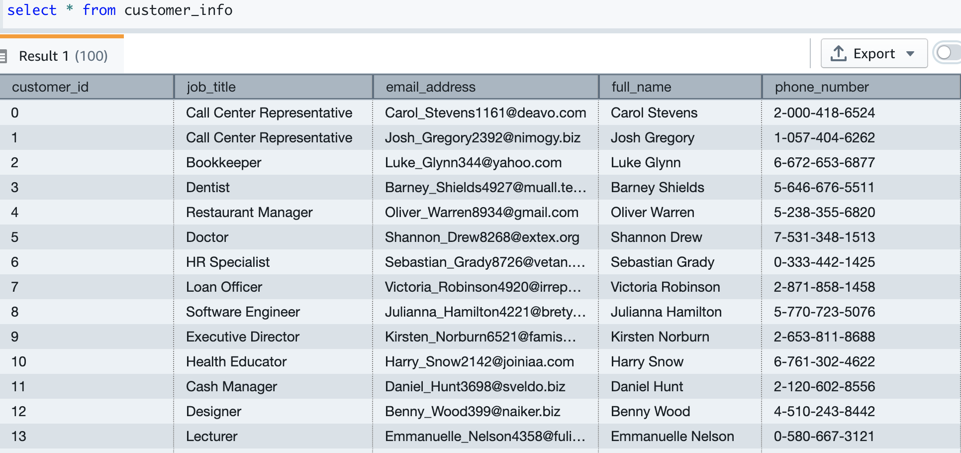
Create and cargo buyer information

Now we create the shopper desk and cargo information, which comprises the e-mail and telephone variety of the shopper. The next code creates the desk, hundreds the information, and samples the desk. The desk DDL is offered on GitHub.

CREATE TABLE public."customer_info"(customer_id bigint NOT NULL encode az64,
job_title character various(500) encode lzo,
email_address character various(100) encode lzo,
full_name character various(200) encode lzo,
phone_number character various(20) encode lzo,
metropolis varchar(50),
state varchar(50)
);
COPY customer_info
FROM 's3://redshift-demos/redshiftml-reinvent/2022/ant312/customer-data/Customer_Data.csv'
IGNOREHEADER 1
IAM_ROLE default CSV;
Choose rely(1) from customer_info;

Our take a look at information has about 5,000 prospects. The next screenshot exhibits pattern buyer information.

Construct an ML mannequin

Our historic card transaction desk has 6 months of information, which we now use to coach and take a look at the ML mannequin.

The mannequin takes the next fields as enter:

TX_DURING_WEEKEND ,
TX_AMOUNT,
TX_DURING_NIGHT ,
CUSTOMER_ID_NB_TX_1DAY_WINDOW ,
CUSTOMER_ID_AVG_AMOUNT_1DAY_WINDOW ,
CUSTOMER_ID_NB_TX_7DAY_WINDOW ,
CUSTOMER_ID_AVG_AMOUNT_7DAY_WINDOW ,
CUSTOMER_ID_NB_TX_30DAY_WINDOW ,
CUSTOMER_ID_AVG_AMOUNT_30DAY_WINDOW ,
TERMINAL_ID_NB_TX_1DAY_WINDOW ,
TERMINAL_ID_RISK_1DAY_WINDOW ,
TERMINAL_ID_NB_TX_7DAY_WINDOW ,
TERMINAL_ID_RISK_7DAY_WINDOW ,
TERMINAL_ID_NB_TX_30DAY_WINDOW ,
TERMINAL_ID_RISK_30DAY_WINDOW

We get tx_fraud as output.

We break up this information into coaching and take a look at datasets. Transactions from 2022-04-01 to 2022-07-31 are for the coaching set. Transactions from 2022-08-01 to 2022-09-30 are used for the take a look at set.

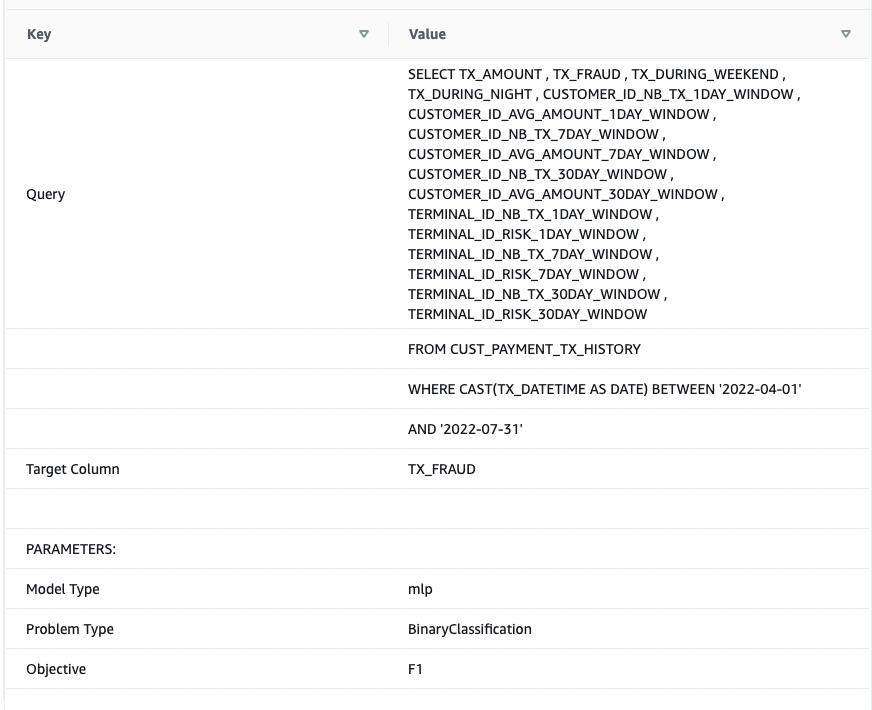
Let’s create the ML mannequin utilizing the acquainted SQL CREATE MODEL assertion. We use a primary type of the Redshift ML command. The next technique makes use of Amazon SageMaker Autopilot, which performs information preparation, function engineering, mannequin choice, and coaching routinely for you. Present the identify of your S3 bucket containing the code.

CREATE MODEL cust_cc_txn_fd
FROM (
SELECT TX_AMOUNT ,
TX_FRAUD ,
TX_DURING_WEEKEND ,
TX_DURING_NIGHT ,
CUSTOMER_ID_NB_TX_1DAY_WINDOW ,
CUSTOMER_ID_AVG_AMOUNT_1DAY_WINDOW ,
CUSTOMER_ID_NB_TX_7DAY_WINDOW ,
CUSTOMER_ID_AVG_AMOUNT_7DAY_WINDOW ,
CUSTOMER_ID_NB_TX_30DAY_WINDOW ,
CUSTOMER_ID_AVG_AMOUNT_30DAY_WINDOW ,
TERMINAL_ID_NB_TX_1DAY_WINDOW ,
TERMINAL_ID_RISK_1DAY_WINDOW ,
TERMINAL_ID_NB_TX_7DAY_WINDOW ,
TERMINAL_ID_RISK_7DAY_WINDOW ,
TERMINAL_ID_NB_TX_30DAY_WINDOW ,
TERMINAL_ID_RISK_30DAY_WINDOW
FROM cust_payment_tx_history
WHERE solid(tx_datetime as date) between '2022-06-01' and '2022-09-30'
) TARGET tx_fraud
FUNCTION fn_customer_cc_fd
IAM_ROLE default
SETTINGS (
S3_BUCKET '<change this together with your s3 bucket identify>',
s3_garbage_collect off,
max_runtime 3600
);

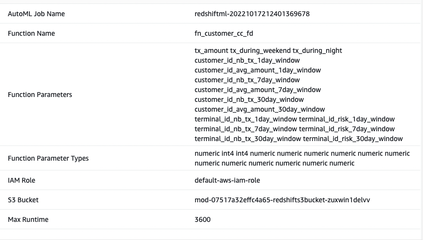
I name the ML mannequin as Cust_cc_txn_fd, and the prediction operate as fn_customer_cc_fd. The FROM clause exhibits the enter columns from the historic desk public.cust_payment_tx_history. The goal parameter is about to tx_fraud, which is the goal variable that we’re attempting to foretell. IAM_Role is about to default as a result of the cluster is configured with this function; if not, you need to present your Amazon Redshift cluster IAM function ARN. I set the max_runtime to three,600 seconds, which is the time we give to SageMaker to finish the method. Redshift ML deploys the perfect mannequin that’s recognized on this timeframe.

Relying on the complexity of the mannequin and the quantity of information, it could actually take a while for the mannequin to be accessible. When you discover your mannequin choice shouldn’t be finishing, enhance the worth for max_runtime. You may set a max worth of 9999.

The CREATE MODEL command is run asynchronously, which implies it runs within the background. You need to use the SHOW MODEL command to see the standing of the mannequin. When the standing exhibits as Prepared, it means the mannequin is skilled and deployed.

present mannequin cust_cc_txn_fd;

The next screenshots present our output.

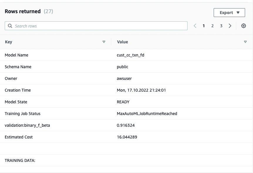
From the output, I see that the mannequin has been accurately acknowledged as BinaryClassification, and F1 has been chosen as the target. The F1 rating is a metric that considers each precision and recall. It returns a worth between 1 (good precision and recall) and 0 (lowest doable rating). In my case, it’s 0.91. The upper the worth, the higher the mannequin efficiency.

Let’s take a look at this mannequin with the take a look at dataset. Run the next command, which retrieves pattern predictions:

SELECT
tx_fraud ,
fn_customer_cc_fd(
TX_AMOUNT ,
TX_DURING_WEEKEND ,
TX_DURING_NIGHT ,
CUSTOMER_ID_NB_TX_1DAY_WINDOW ,
CUSTOMER_ID_AVG_AMOUNT_1DAY_WINDOW ,
CUSTOMER_ID_NB_TX_7DAY_WINDOW ,
CUSTOMER_ID_AVG_AMOUNT_7DAY_WINDOW ,
CUSTOMER_ID_NB_TX_30DAY_WINDOW ,
CUSTOMER_ID_AVG_AMOUNT_30DAY_WINDOW ,
TERMINAL_ID_NB_TX_1DAY_WINDOW ,
TERMINAL_ID_RISK_1DAY_WINDOW ,
TERMINAL_ID_NB_TX_7DAY_WINDOW ,
TERMINAL_ID_RISK_7DAY_WINDOW ,
TERMINAL_ID_NB_TX_30DAY_WINDOW ,
TERMINAL_ID_RISK_30DAY_WINDOW )
FROM cust_payment_tx_history
WHERE solid(tx_datetime as date) >= '2022-10-01'
restrict 10 ;

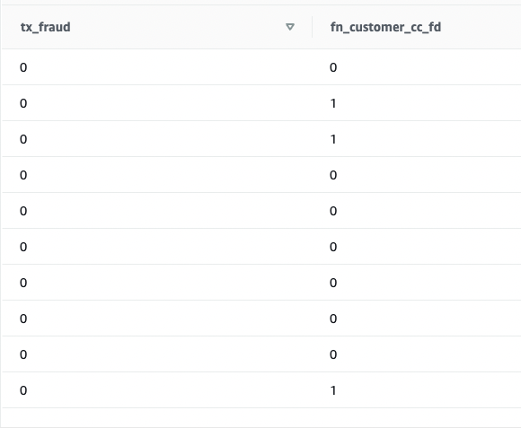
We see that some values are matching and a few aren’t. Let’s examine predictions to the bottom reality:

SELECT
tx_fraud ,
fn_customer_cc_fd(
TX_AMOUNT ,
TX_DURING_WEEKEND ,
TX_DURING_NIGHT ,
CUSTOMER_ID_NB_TX_1DAY_WINDOW ,
CUSTOMER_ID_AVG_AMOUNT_1DAY_WINDOW ,
CUSTOMER_ID_NB_TX_7DAY_WINDOW ,
CUSTOMER_ID_AVG_AMOUNT_7DAY_WINDOW ,
CUSTOMER_ID_NB_TX_30DAY_WINDOW ,
CUSTOMER_ID_AVG_AMOUNT_30DAY_WINDOW ,
TERMINAL_ID_NB_TX_1DAY_WINDOW ,
TERMINAL_ID_RISK_1DAY_WINDOW ,
TERMINAL_ID_NB_TX_7DAY_WINDOW ,
TERMINAL_ID_RISK_7DAY_WINDOW ,
TERMINAL_ID_NB_TX_30DAY_WINDOW ,
TERMINAL_ID_RISK_30DAY_WINDOW
) as prediction, rely(*) as values
FROM public.cust_payment_tx_history
WHERE solid(tx_datetime as date) >= '2022-08-01'
Group by 1,2 ;

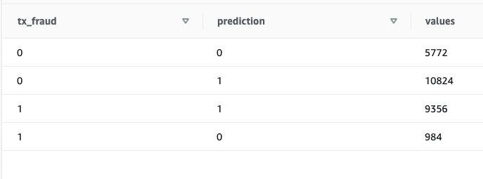
We validated that the mannequin is working and the F1 rating is sweet. Let’s transfer on to producing predictions on streaming information.

Predict fraudulent transactions

As a result of the Redshift ML mannequin is able to use, we are able to use it to run the predictions towards streaming information ingestion. The historic dataset has extra fields than what we’ve got within the streaming information supply, however they’re simply recency and frequency metrics across the buyer and terminal danger for a fraudulent transaction.

We are able to apply the transformations on prime of the streaming information very simply by embedding the SQL contained in the views. Create the first view, which aggregates streaming information on the buyer degree. Then create the second view, which aggregates streaming information at terminal degree, and the third view, which mixes incoming transactional information with buyer and terminal aggregated information and calls the prediction operate multi functional place. The code for the third view is as follows:

CREATE VIEW public.cust_payment_tx_fraud_predictions
as
choose a.approximate_arrival_timestamp,
d.full_name , d.email_address, d.phone_number,
a.TRANSACTION_ID, a.TX_DATETIME, a.CUSTOMER_ID, a.TERMINAL_ID,
a.TX_AMOUNT ,
a.TX_TIME_SECONDS ,
a.TX_TIME_DAYS ,
public.fn_customer_cc_fd(a.TX_AMOUNT ,
a.TX_DURING_WEEKEND,
a.TX_DURING_NIGHT,
c.CUSTOMER_ID_NB_TX_1DAY_WINDOW ,
c.CUSTOMER_ID_AVG_AMOUNT_1DAY_WINDOW ,
c.CUSTOMER_ID_NB_TX_7DAY_WINDOW ,
c.CUSTOMER_ID_AVG_AMOUNT_7DAY_WINDOW ,
c.CUSTOMER_ID_NB_TX_30DAY_WINDOW ,
c.CUSTOMER_ID_AVG_AMOUNT_30DAY_WINDOW ,
t.TERMINAL_ID_NB_TX_1DAY_WINDOW ,
t.TERMINAL_ID_RISK_1DAY_WINDOW ,
t.TERMINAL_ID_NB_TX_7DAY_WINDOW ,
t.TERMINAL_ID_RISK_7DAY_WINDOW ,
t.TERMINAL_ID_NB_TX_30DAY_WINDOW ,
t.TERMINAL_ID_RISK_30DAY_WINDOW ) Fraud_prediction
From
(choose
Approximate_arrival_timestamp,
TRANSACTION_ID, TX_DATETIME, CUSTOMER_ID, TERMINAL_ID,
TX_AMOUNT ,
TX_TIME_SECONDS ,
TX_TIME_DAYS ,
case when extract(dow from solid(TX_DATETIME as timestamp)) in (1,7) then 1 else 0 finish as TX_DURING_WEEKEND,
case when extract(hour from solid(TX_DATETIME as timestamp)) between 00 and 06 then 1 else 0 finish as TX_DURING_NIGHT
FROM cust_payment_tx_stream) a
be a part of terminal_transformations t
on a.terminal_id = t.terminal_id
be a part of customer_transformations c
on a.customer_id = c.customer_id
be a part of customer_info d
on a.customer_id = d.customer_id
;

Run a SELECT assertion on the view:

choose * from
cust_payment_tx_fraud_predictions
the place Fraud_prediction = 1;

As you run the SELECT assertion repeatedly, the most recent bank card transactions undergo transformations and ML predictions in near-real time.

This demonstrates the ability of Amazon Redshift—with easy-to-use SQL instructions, you’ll be able to rework streaming information by making use of complicated window capabilities and apply an ML mannequin to foretell fraudulent transactions multi functional step, with out constructing complicated information pipelines or constructing and managing further infrastructure.

Broaden the answer

As a result of the information streams in and ML predictions are made in near-real time, you’ll be able to construct enterprise processes for alerting your buyer utilizing Amazon Easy Notification Service (Amazon SNS), or you’ll be able to lock the shopper’s bank card account in an operational system.

This submit doesn’t go into the main points of those operations, however in case you’re concerned about studying extra about constructing event-driven options utilizing Amazon Redshift, confer with the next GitHub repository.

Clear up

To keep away from incurring future costs, delete the sources that had been created as a part of this submit.

Conclusion

On this submit, we demonstrated learn how to arrange a Kinesis information stream, configure a producer and publish information to streams, after which create an Amazon Redshift Streaming Ingestion view and question the information in Amazon Redshift. After the information was within the Amazon Redshift cluster, we demonstrated learn how to practice an ML mannequin and construct a prediction operate and apply it towards the streaming information to generate predictions near-real time.

When you have any suggestions or questions, please depart them within the feedback.

Concerning the Authors

Bhanu Pittampally is an Analytics Specialist Options Architect based mostly out of Dallas. He focuses on constructing analytic options. His background is in information warehouses—structure, growth, and administration. He has been within the information and analytics subject for over 15 years.

Praveen Kadipikonda is a Senior Analytics Specialist Options Architect at AWS based mostly out of Dallas. He helps prospects construct environment friendly, performant, and scalable analytic options. He has labored with constructing databases and information warehouse options for over 15 years.

Ritesh Kumar Sinha is an Analytics Specialist Options Architect based mostly out of San Francisco. He has helped prospects construct scalable information warehousing and massive information options for over 16 years. He likes to design and construct environment friendly end-to-end options on AWS. In his spare time, he loves studying, strolling, and doing yoga.