Create, Prepare and Deploy Multi Layer Perceptron (MLP) fashions utilizing Amazon Redshift ML

Amazon Redshift is a totally managed and petabyte-scale cloud knowledge warehouse which is being utilized by tens of hundreds of shoppers to course of exabytes of information daily to energy their analytics workloads. Amazon Redshift comes with a function referred to as Amazon Redshift ML which places the ability of machine studying within the fingers of each knowledge warehouse consumer, with out requiring the customers to be taught any new programming language, ML ideas or ML instruments. Redshift ML abstracts all of the intricacies which can be concerned within the conventional ML strategy round knowledge warehouse which historically concerned repetitive, guide steps to maneuver knowledge backwards and forwards between the information warehouse and ML instruments for working lengthy, complicated, iterative ML workflow.

Redshift ML makes use of Amazon SageMaker Autopilot and Amazon SageMaker Neo within the background to make it simple for SQL customers comparable to knowledge analysts, knowledge scientists, BI specialists and database builders to create, prepare, and deploy machine studying (ML) fashions utilizing acquainted SQL instructions after which use these fashions to make predictions on new knowledge to be used instances comparable to buyer churn prediction, basket evaluation for gross sales prediction, manufacturing unit lifetime worth prediction, and product suggestions. Redshift ML makes the mannequin obtainable as SQL perform inside the Amazon Redshift knowledge warehouse so you may simply use it in queries and studies.

Amazon Redshift ML helps supervised studying, together with regression, binary classification, multi-class classification, and unsupervised studying utilizing Ok-Means. You may optionally specify XGBoost, MLP, and linear learner mannequin sorts, that are supervised studying algorithms used for fixing both classification or regression issues, and supply a big improve in pace over conventional hyperparameter optimization strategies. Amazon Redshift ML additionally helps bring-your-own-model to both import present SageMaker fashions which can be constructed utilizing algorithms supported by SageMaker Autopilot, which can be utilized for native inference; or for the unsupported algorithms, one can alternatively invoke distant SageMaker endpoints for distant inference.

On this weblog publish, we present you the best way to use Redshift ML to resolve binary classification downside utilizing the Multi Layer Perceptron (MLP) algorithm, which explores totally different coaching aims and chooses one of the best answer from the validation set.

A multilayer perceptron (MLP) is a deep studying technique which offers with coaching multi-layer synthetic neural networks, additionally referred to as Deep Neural Networks. It’s a feedforward synthetic neural community that generates a set of outputs from a set of inputs. An MLP is characterised by a number of layers of enter nodes linked as a directed graph between the enter and output layers. MLP makes use of backpropagation for coaching the community. MLP is extensively used for fixing issues that require supervised studying in addition to analysis into computational neuroscience and parallel distributed processing. It is usually used for speech recognition, picture recognition and machine translation.

So far as MLP utilization with Redshift ML (powered by Amazon SageMaker Autopilot) is worried, it helps tabular knowledge as of now.

Resolution Overview

To make use of the MLP algorithm, it’s essential to present inputs or columns representing dimensional values and in addition the label or goal, which is the worth you’re attempting to foretell.

With Redshift ML, you need to use MLP on tabular knowledge for regression, binary classification or multiclass classification issues. What’s extra distinctive about MLP is, is that the output perform of MLP generally is a linear or a steady perform as effectively. It needn’t be a straight line like the overall regression mannequin offers.

On this answer, we use binary classification to detect frauds primarily based upon the bank cards transaction knowledge. The distinction between classification fashions and MLP is that logistic regression makes use of a logistic perform, whereas perceptrons use a step perform. Utilizing the multilayer perceptron mannequin, machines can be taught weight coefficients that assist them classify inputs. This linear binary classifier is very efficient in arranging and categorizing enter knowledge into totally different courses, permitting probability-based predictions and classifying gadgets into a number of classes. Multilayer Perceptrons have the benefit of studying non-linear fashions and the flexibility to coach fashions in real-time.

For this answer, we first ingest the information into Amazon Redshift, we then distribute it for mannequin coaching and validation, then use Amazon Redshift ML particular queries for mannequin creation and thereby create and make the most of the generated SQL perform for with the ability to lastly predict the fraudulent transactions.

Conditions

To get began, we’d like an Amazon Redshift cluster or an Amazon Redshift Serverless endpoint and an AWS Identification and Entry Administration (IAM) function hooked up that gives entry to SageMaker and permissions to an Amazon Easy Storage Service (Amazon S3) bucket.

For an introduction to Redshift ML and directions on setting it up, see Create, prepare, and deploy machine studying fashions in Amazon Redshift utilizing SQL with Amazon Redshift ML.

To create a easy cluster with a default IAM function, see Use the default IAM function in Amazon Redshift to simplify accessing different AWS providers.

Information Set Used

On this publish, we use the Credit score Card Fraud detection knowledge to create, prepare and deploy MLP mannequin which can be utilized additional to establish fraudulent transactions from the newly captured transaction data.

The dataset accommodates transactions made by bank cards in September 2013 by European cardholders.
This dataset presents transactions that occurred in two days, the place we now have 492 frauds out of 284,807 transactions. The dataset is very unbalanced, the constructive class (frauds) account for 0.172% of all transactions.

It accommodates solely numerical enter variables that are the results of a Principal Part Evaluation transformation. Resulting from confidentiality points, the unique options and extra background details about the information is just not supplied. Options V1, V2, … V28 are the principal elements obtained with PCA, the one options which haven’t been remodeled with PCA are ‘Time’ and ‘Quantity’. Characteristic ‘Time’ accommodates the seconds elapsed between every transaction and the primary transaction within the dataset. The function ‘Quantity’ is the transaction Quantity. Characteristic ‘Class’ is the response variable and it takes worth 1 in case of fraud and 0 in any other case.

Listed below are pattern data:

Put together the information

Load the bank card dataset into Amazon Redshift utilizing the next SQL. You should use the Amazon Redshift question editor v2 or your most popular SQL instrument to run these instructions.

To create the desk, use the next command:

CREATE TABLE creditcardsfrauds (
    txtime integer,
    v1 float8,
    v2 float8,
    v3 float8,
    v4 float8,
    v5 float8,
    v6 float8,
    v7 float8,
    v8 float8,
    v9 float8,
    v10 float8,
    v11 float8,
    v12 float8,
    v13 float8,
    v14 float8,
    v15 float8,
    v16 float8,
    v17 float8,
    v18 float8,
    v19 float8,
    v20 float8,
    v21 float8,
    v22 float8,
    v23 float8,
    v24 float8,
    v25 float8,
    v26 float8,
    v27 float8,
    v28 float8,
    quantity float8,
    class integer
);

Load the information

To load knowledge into Amazon Redshift, use the next COPY command:

COPY creditcardsfrauds
FROM 's3://redshift-ml-blog-mlp/creditcard.csv' 
IAM_ROLE default
CSV QUOTE as '"' delimiter ',' IGNOREHEADER 1 maxerror 100
REGION 'us-east-1';

Earlier than creating the mannequin, we need to divide our knowledge into two units by splitting 80% of the dataset for coaching and 20% for validation, which is a typical follow in ML. The coaching knowledge is enter to the ML mannequin to establish the absolute best algorithm for the mannequin. After the mannequin is created, we use the validation knowledge to validate the mannequin accuracy.

So, in ‘creditcardsfrauds’ desk, we examine the distribution of information primarily based upon ‘txtime’ worth and establish the cutoff for round 80% of the information to coach the mannequin.

With this, the very best txtime worth involves 120954 (primarily based upon the distribution of txtime’s min, max, rating by window perform and ceil(depend(*)*0.80) values)), primarily based upon which we think about the transaction data having ‘txtime’ subject worth lower than 120954 for creating coaching knowledge. We then validate the accuracy of that mannequin by seeing if it accurately identifies the fraudulent transactions by predicting its ‘class’ attribute on the remaining 20% of the information.

This distribution for 80% cutoff needn’t all the time be primarily based upon ordered time. It may be picked up randomly as effectively, primarily based upon the use case into account.

Create a mannequin in Redshift ML

To create the mannequin, use the next command:

 CREATE mannequin creditcardsfrauds_mlp
FROM (choose * from creditcardsfrauds the place txtime < 120954)
TARGET class 
FUNCTION creditcardsfrauds_mlp_fn
IAM_ROLE default
MODEL_TYPE MLP
SETTINGS (
      S3_BUCKET '<<your-amazon-s3-bucket-name>>’,
      MAX_RUNTIME 9600
);

Right here, within the settings part of the command, it’s essential to arrange an S3_BUCKET which is used to export the information that’s despatched to SageMaker and retailer mannequin artifacts.

S3_BUCKET setting is a required parameter of the command, whereas MAX_RUNTIME is an non-compulsory one which specifies the utmost period of time to coach. The default worth of this parameter is 90 minutes (5400 seconds), nevertheless you may override it by explicitly specifying it within the command, identical to we now have achieved it right here by setting it to run for 9600 seconds.

The previous assertion initiates an Amazon SageMaker Autopilot course of within the background to routinely construct, prepare, and tune one of the best ML mannequin for the enter knowledge. It then makes use of Amazon SageMaker Neo to deploy that mannequin regionally within the Amazon Redshift cluster or Amazon Redshift Serverless as a user-defined perform (UDF).

You should use the SHOW MODEL command in Amazon Redshift to trace the progress of your mannequin creation, which must be within the READY state inside the max_runtime parameter you outlined whereas creating the mannequin.

To examine the standing of the mannequin, use the next command:

present mannequin creditcardsfrauds_mlp;

We discover from the previous desk that the F1-score for the coaching knowledge is 0.908, which reveals superb efficiency accuracy.

To elaborate, F1-score is the harmonic imply of precision and recall. It combines precision and recall right into a single quantity utilizing the next components:

The place, Precision means: Of all constructive predictions, what number of are actually constructive?

And Recall means: Of all actual constructive instances, what number of are predicted constructive?

F1 scores can vary from 0 to 1, with 1 representing a mannequin that completely classifies every commentary into the proper class and 0 representing a mannequin that’s unable to categorise any commentary into the proper class. So larger F1 scores are higher.

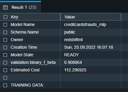
The next is the detailed tabular final result for the previous command after mannequin coaching was achieved.

Redshift ML now helps Prediction Chances for binary classification fashions. For classification downside in machine studying, for a given document, every label may be related to a likelihood that signifies how doubtless this document actually belongs to the label. With choice to have chances together with the label, clients might use the classification outcomes when confidence primarily based on chosen label is larger than a sure threshold worth returned by the mannequin

Prediction chances are calculated by default for binary classification fashions and a further perform is created whereas creating mannequin with out impacting efficiency of the ML mannequin.

In above snippet, you’ll discover that predication chances enhancements have added one other perform as a suffix (_prob) to mannequin perform with a reputation ‘creditcardsfrauds_mlp_fn_prob’ which may very well be used to get prediction chances.

Moreover, you may examine the mannequin explainability to grasp which inputs contributed successfully to derive the prediction.

Mannequin explainability helps to grasp the reason for prediction by answering questions comparable to:

• Why did the mannequin predict a unfavourable final result comparable to blocking of bank card when somebody travels to a special nation and withdraws some huge cash in several foreign money?
• How does the mannequin make predictions? Plenty of knowledge for bank cards may be put in a tabular format and as per MLP course of the place a totally linked neural community of a number of layers is concerned, we are able to inform which enter function really contributed to the mannequin output and its magnitude.
• Why did the mannequin make an incorrect prediction? E.g. Why is the cardboard blocked despite the fact that the transaction is official?
• Which options have the most important affect on the habits of the mannequin? Is it simply primarily based upon the situation the place the bank card is swiped, and even the time of the day and weird credit score consumption that’s influencing the prediction?

Run the next SQL command to retrieve the values from the explainability report:

SELECT json_table.report.explanations.kernel_shap.label0.global_shap_values 
FROM (choose explain_model('creditcardsfrauds_mlp') as report) as json_table;

Within the previous screenshot, we now have solely chosen the column that initiatives shapley values from the response returned by the explain_model perform. When you discover the response of the question, the values in each json object present the contribution of various options when it comes to influencing the prediction. E.g. from the previous snippet, v14 function is influencing the prediction probably the most and txtime function does probably not play any vital function in predicting ‘class’.

Mannequin validation

Now let’s run the prediction question and validate the accuracy of the mannequin on the validation dataset:

FROM (
  SELECT 
      CASE WHEN class =  
      creditcardsfrauds_mlp_fn(txtime,v1,v2,v3,v4,v5,v6,v7,v8,v9,v10,v11,v12,v13,v14,v15,v16,v17,v18,v19,v20,v21,v22,v23,v24,v25,v26,v27,v28,quantity) 
      THEN 'PredictedMatchesActual' 
      else 'NoMatch' 
      END as actualvspredicted
    FROM creditcardsfrauds 
    WHERE txtime >= 120954
) 
group by actualvspredicted

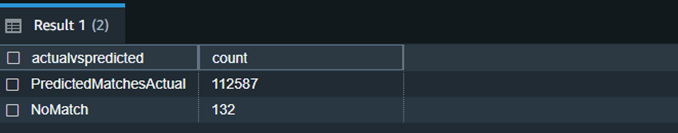
We will observe right here that Redshift ML is ready to establish 99.88 % of the transactions accurately as fraudulent or non-fraudulent.

Now you may proceed to make use of this SQL perform creditcardsfrauds_mlp_fn for native inference in any a part of the SQL question whereas analyzing, visualizing or reporting the newly arriving in addition to present knowledge!

--CREATE A STAGING TABLE TO HOLD NEWLY ARRIVING DATA FROM THE SOURCE WHICH WILL NOT CONAIN THE CLASS COLUMN - AS IT IS TO BE PREDICTED
DROP TABLE creditcardsfrauds_staging;
CREATE TABLE creditcardsfrauds_staging as (choose * from creditcardsfrauds restrict 0);
Alter desk creditcardsfrauds_staging drop column class;

--LETS CONSIDER ONLY ONE RECORD HERE WHICH HAS NEWLY ARRIVED
insert into creditcardsfrauds_staging values(174965,-39999.11383160738512,0.58586417180689,-5.39973021073242,1.81709247345531,-0.840618465991056,-2.94354779071974,-2.20800192003372,1.05873267723056,-1.63233334974982,-5000.24598383776964,11.93351953683592,-53046479695456,-1.12745457501155,-666666.41662797597451,0.141237234328704,-2.54949823633632,-4.61471706851594,-10.47813794126038,-0.0354803664667244,0.306270740368093,0.583275998701341,-0.269208637986581,-0.456107772584008,-0.183659129549716,-0.328167759255761,0.606115810329683,0.884875539542905,-0.253700318894381,-2450000000);

--USE THE FUNCTION TO PREDICT THE VALUE OF CLASS
SELECT txtime, creditcardsfrauds_mlp_fn(txtime,v1,v2,v3,v4,v5,v6,v7,v8,v9,v10,v11,v12,v13,v14,v15,v16,v17,v18,v19,v20,v21,v22,v23,v24,v25,v26,v27,v28,quantity)
FROM creditcardsfrauds_staging;

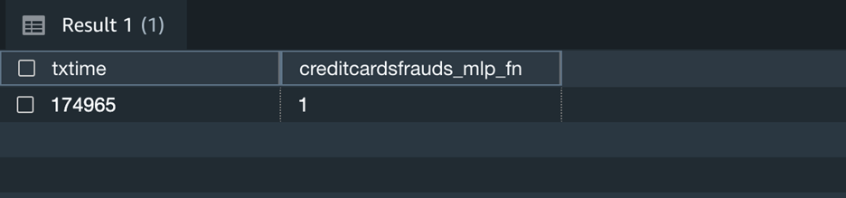
Right here the output 1 implies that the newly captured transaction is fraudulent as per the inference.

Moreover, you may change the above question to incorporate prediction chances of label output for the above state of affairs and determine when you nonetheless like to make use of the prediction by the mannequin.

--USE THE FUNCTION TO PREDICT THE VALUE OF CLASS ALONG WITH THE PROBABILITY
Choose txtime, predictedActive.labels[0], predictedActive.chances[0] 
from (
SELECT txtime, creditcardsfrauds_mlp_fn_prob(txtime,v1,v2,v3,v4,v5,v6,v7,v8,v9,v10,v11,v12,v13,v14,v15,v16,v17,v18,v19,v20,v21,v22,v23,v24,v25,v26,v27,v28,quantity)as predictedACtive
FROM creditcardsfrauds_staging ) temp

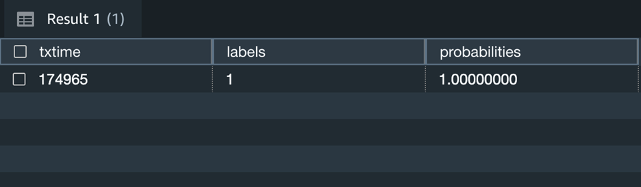
The above screenshot reveals that this transaction has 100% probability of being fraudulent.

Clear up

To keep away from incurring future fees, you may cease the Redshift cluster when not getting used. You may even terminate the Redshift cluster altogether if in case you have run the train on this weblog publish only for experimental function. If you’re as an alternative utilizing serverless model of Redshift, it won’t value you something, till it’s used. Nonetheless, like talked about earlier than, you’ll have to cease or terminate the cluster if you’re utilizing a provisioned model of Redshift.

Conclusion

Redshift ML makes it simple for customers of all ranges to create, prepare, and tune fashions utilizing SQL interface. On this publish, we walked you thru the best way to use the MLP algorithm to create binary classification mannequin. You may then use these fashions to make predictions utilizing easy SQL instructions and achieve precious insights.

To be taught extra about RedShift ML, go to Amazon Redshift ML.

In regards to the authors

Anuradha Karlekar is a Options Architect at AWS working majorly for Companions and Startups. She has over 15 years of IT expertise extensively in full stack growth, deployment, constructing knowledge ETL pipelines and visualizations. She is obsessed with knowledge analytics and textual content search. Outdoors work – She is a journey fanatic!

Phil Bates is a Senior Analytics Specialist Options Architect at AWS with over 25 years of information warehouse expertise.

Abhishek Pan is a Options Architect-Analytics working at AWS India. He engages with clients to outline knowledge pushed technique, present deep dive periods on analytics use instances & design  scalable and performant Analytical purposes. He has over 11 years of expertise and is obsessed with Databases, Analytics and fixing buyer issues with assist of cloud options. An avid traveller and tries to seize world by my lenses

Debu Panda is a Senior Supervisor, Product Administration at AWS, is an business chief in analytics, utility platform, and database applied sciences, and has greater than 25 years of expertise within the IT world. Debu has revealed quite a few articles on analytics, enterprise Java, and databases and has offered at a number of conferences comparable to re:Invent, Oracle Open World, and Java One. He’s lead creator of the EJB 3 in Motion (Manning Publications 2007, 2014) and Middleware Administration (Packt).